
Who sets your bifacial factors?
Every bifacial yield forecast in PVsyst rests on correction factors no one can measure, so someone has to supply them, and someone eventually has to defend them. This page sets out where those factors come from, why every system needs its own set, and what to ask of anyone who provides them.
PVsyst needs bifacial inputs no one can measure
PVsyst, like most yield programs, models rear-side light with a simple optical model called the view factor model. It solves the optics of an ideal system: no structural supports, no gaps between modules or bays, one uniform ground, and no dependence on wavelength. For that ideal system it is accurate, and agrees closely with ray tracing.
Real systems break every one of those assumptions, and the accuracy goes with them. To recover it, the program applies four correction factors, usually called bifacial factors. Three of them cannot be measured at all: they describe how a specific structure, module and site interact with light, and the only way to obtain them is to simulate that interaction in more detail than the view factor model allows.
The fourth, albedo, can be measured, but only as a single broadband number. The ground reflects each wavelength differently and the spectrum falling on it changes through the day and year, so the light actually reaching the rear cells is not what that one number implies. Each of the four factors carries considerably more physics than its name suggests.
Structure shading factor
fSShading and reflection from torque tubes, posts, rails, gearboxes and cabling.
Shed transparent fraction
fTLight passing through and between modules onto the ground, and the extra light reaching modules at row ends and array edges.
Ground albedo
fAOne broadband number standing in for a ground that reflects each wavelength differently, under a spectrum that changes through the day and year.
Rear mismatch loss
fMRThe electrical loss from non-uniform rear irradiance, including non-uniformity within a single module.
Four factors therefore stand in for three-dimensional geometry, a varying spectrum and the electrical behaviour of the module, none of which the view factor model represents directly. The accuracy of a bifacial yield model rests on inputs it cannot check and cannot warn you about when they are wrong.
The three structural and electrical factors cannot be measured. Isolating the shading contribution of a torque tube, or the electrical mismatch from rear non-uniformity, would mean building the same array twice, changing one component, and holding the weather identical for long enough to separate that effect from everything else moving around it. In practice that is virtually impossible: the weather cannot be held constant, and a tracker cannot be built without the structural supports whose shading you are trying to measure. So the factors are simulated.
If the factors have to be simulated, can a default value, or one borrowed from another project, stand in for them?
Every system has its own set of factors
Change only the module, holding site and tracker constant, and the structure shading factor moves substantially. Change only the site, holding the design constant, and rear mismatch moves substantially.
The same LR5 module gives 13.4% on a 1P tracker and 10.1% on a 2P. That is 3.3 percentage points from the structure alone. Within one architecture, changing only the module moves it by up to 2.6 points.
Virginia and Brazil have an identical diffuse fraction of 40.9% and sit 2.1 percentage points apart. Latitude does not order the results either. No single site statistic predicts the factor.
Each factor belongs to one specific combination of structure, module and site. Change any one of them and the right value changes with it.
$105,000 a year 0.3% of annual yield on a 500 MW project at a 20% capacity factor and $40/MWh. Structural factors off by 5 to 8 percentage points move total yield by that much, and a 5% default where the real value is nearer 10% is exactly that size of error.
“The SunSolve process, using ray-tracing, provides the level of precision that's required — for multi gigawatt-scale projects, in particular. If there's a 1% error, it's going to have a much bigger impact in dollar terms on a multi-gigawatt scale project. These errors become very, very impactful. Trying to resolve them is worth a lot of money.”
Comparing two systems needs the same method for both
A developer receives factors for tracker A from one source and factors for tracker B from another. Both go into PVsyst, and the difference in the output is read as a difference in hardware. Part of it is. The rest is the difference between the two methods that produced the factors, and nothing in PVsyst shows which part is which.
The methods in common use differ in ways that can move the factors by as much as the hardware does. Whether the torque tube and posts are modelled or approximated, whether module frames are included, how much detail the module itself is given, whether the spectrum is resolved or a broadband albedo is used. Each choice can shift a factor by a percentage point or more, which is the same order as the difference between two alternative trackers. The same tool is not enough; it has to be the same method, at the same level of detail, applied to both.
Applying the same method to both trackers removes that noise, and the difference in PVsyst becomes a difference in hardware again. But a consistent method is only the first requirement. If the method itself leaves out the structure, ignores light that reaches the rear after more than one bounce, or assumes a fixed spectrum, both sets of factors are wrong in the same way, and the comparison is fair but the yield is not. The following sections set out a method that is both.
“The industry has players that have exaggerated yield claims and we want real numbers. The closest to reality is what SunSolve delivers. Nextpower prides itself on being very technically competent and technically driven and in trusting the scientific results. We just want the right answer. SunSolve is the best and the most technically competent.”
From solar cell to solar farm, one physics engine
SunSolve was originally built to serve the cell and module manufacturing industry, where fierce competition drives a constant innovation cycle. Predictions are checked against laboratory measurements every day, in highly controlled environments where the inputs are known and the device can be measured directly. The models are under constant scrutiny.
Laboratory and field validation answer different questions. In the laboratory, it is far easier to design a controlled, repeatable experiment, so predictions can be compared against measurement with low uncertainty.
In the field, weather, spectrum, soiling and albedo all change during the experiment, and the combined measurement uncertainty can be comparable to the effects being studied. A well-designed field experiment tests the model under real operating conditions, but even then the signal from any single effect can be difficult to distinguish from the noise. SunSolve's engine has been tested in both settings: in the laboratory by leading cell and module manufacturers and in more than 100 published papers, and in the field by some of the world's largest utility-scale developers, EPCs and equipment manufacturers. That combination is what makes SunSolve unique.
Published papers have applied and tested the SunSolve engine.
LONGi used SunSolve to compare simulation against measurement for their world-record heterojunction cell.
The system model uses the same optical and electrical physics as the cell model, extended to system scale, rather than a system model retrofitted with cell detail.
The same physics from cell to system — that is how SunSolve sees the bifacial gains other software can't.
How closely the simulation follows reality
SunSolve models the tracker as it is built and follows how each component interacts with light.
The structure is modelled as it is built
Actual torque tube profile and position, posts, clamps, rails, module frames, motor gaps, bay spacing, row pitch.
The rear shadow is computed from the hardware itself, at each timestep as the tracker turns. A view factor model assumes no structure behind the tracker blocking the rear light, which will overestimate bifacial yield. An overly conservative structure shading factor will underestimate it.
Light is followed from the source, through every bounce, to the cell
Forward ray tracing launches rays from the sun and the surrounding sky dome, following them until they are absorbed or lost, rather than sampling backwards from chosen points.
Second-, third- and higher-order reflections are counted: light bouncing off the ground, off the structure, off a neighbouring row and onto the rear of the next. These paths contribute real rear irradiance. A view factor model cannot represent them at all. A ray tracer that caps its bounce depth, or samples backwards from chosen points, trades accuracy for speed.
The spectrum is resolved at every timestep
An atmospheric model computes the incident spectrum through the year rather than assuming a fixed reference.
Most programs assume a fixed reference spectrum. The spectrum computed for the site captures the seasonal and intraday variation in spectral response, which affects c-Si and CdTe differently.
Every surface has wavelength-dependent optical properties
Ground, steel, glass, encapsulant, cell, backsheet, each with its own reflectance and absorptance across the spectrum.
Ground and structural reflection is resolved wavelength by wavelength against the spectrum actually arriving, so the effective albedo reported back accounts for that interaction rather than a single broadband assumption.
Diffuse light gets the same treatment
Shading is solved separately for every direction in the sky dome, rather than applying one reduction to the whole of it.
Diffuse light reaches the module rear from right across the sky. The structure blocks some of those directions and not others, and the sky is not equally bright in every direction, so how much arrives depends on which part of the sky is blocked. A single reduction factor assumes that does not matter.
Every cell is resolved front and back, then simulated electrically
Front and rear irradiance is computed for each cell, then a circuit solve runs across the module: every cell, how they are wired in series and parallel, and the bypass diodes that switch in and out as the shadow moves.
Cells wired in series are limited to the current of the weakest one, so a shadow falling across a few cells costs far more than its area suggests. Shade more, and a bypass diode activates, a whole substring drops out at once, and the loss jumps rather than sliding. A loss estimated from an irradiance non-uniformity statistic cannot see either of those, because both depend on how the module is wired rather than on how the light is spread.
The whole year is simulated, not sample days
Every timestep, against site weather data. The common shortcut when estimating bifacial factors is to run the solstices and the equinoxes and scale the result up, which captures the range of sun positions and nothing else.
The factor is energy-weighted, and structural shading behaves differently in direct and diffuse light: a hard shadow sweeping across the rear under clear sky, a softer shadow under cloud. The factor depends on how the year divides between the two, which a handful of dates cannot show.
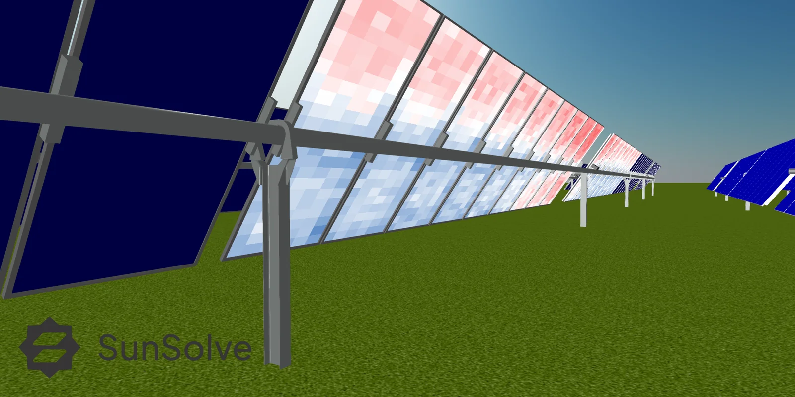
The bifacial factor simulation shown above traces around 43 billion rays at roughly 240 million rays a second.
SunSolve tackles difficult physics with computing power rather than simple approximations.
Independently reviewed and field validated
Independently reviewed
ICF Resources, engaged as independent engineer, has reviewed the SunSolve ray-tracing methodology and the way the four PVsyst bifacial inputs are derived from it. ICF assessed both as “appropriate and consistent with industry-accepted PV modeling practices.”
The independent review was commissioned by Nextpower. It examines the method rather than validating it against a field measurement, and it records the assumptions and limitations of the approach alongside its conclusions.
We can send ICF's report to developers, EPCs, IPPs and independent engineers on request.
Studies using SunSolve Yield
Front and rear irradiance against pyranometers at the torque tube axis and in the plane of array on a 1P tracker, matching both the profile and second-order effects. K. R. McIntosh et al., “The influence of wind and module tilt on the operating temperature of single-axis trackers,” IEEE PVSC 2022, doi:10.1109/PVSC48317.2022.9938577. Read the paper Extracting irradiance from ray tracing with dedicated sensors in SunSolve
The full workflow, from simulation through PVsyst factors to net energy, agreeing within ±0.3% over a 16-day test. Scope stated plainly: one site, one tracker, and the procedure as it stood in 2020. Array described the resulting method as “bankable, real-world modeling best practices for bifacial power plants”. K. Passow et al., “Estimating bifacial loss factors for annual utility scale simulations,” IEEE PVSC 2020, doi:10.1109/PVSC45281.2020.9300403. Read the paper Simulation and Measurement of monofacial and bifacial modules in a 1D tracking system Field testing meets modeling: validated data on bifacial solar performance
Ray tracing and circuit modelling of mismatch loss from nonuniform rear illumination on a 1-D tracker. In the example studied, a one-high configuration at Golden, CO, the annual yield reduction is 0.23% for a central module and 0.35% for an edge module. Simulation only, for one site and configuration. K. R. McIntosh, M. D. Abbott, B. A. Sudbury and J. Meydbray, “Mismatch loss in bifacial modules due to nonuniform illumination in 1-D tracking systems,” IEEE J. Photovoltaics, 2019, doi:10.1109/JPHOTOV.2019.2937217. Read the paper
Predicts bifacial gain for AgriPV layouts using SunSolve ray tracing and PVsyst's factors. The post reports gains from 2% to 50% depending on design. Simulation only; the post notes that experimental validation of AgriPV procedures is still needed. Calculating the bifacial gain of AgriPV systems with SunSolve and PVsyst
A 12-month ray-tracing simulation of a proposed Northern Australia site. Conventional PVsyst predictions showed no bifacial gain; the simulation found 1–2%. How 5B Used Physics-Based Modelling to Unlock Hidden Yield in the Maverick
This is a selection of studies that use SunSolve Yield, not a complete list. For the latest up-to-date listing, please contact us.
Not only PVsyst
The same derivation feeds any yield tool that takes bifacial inputs. PlantPredict imports the factors at every timestep rather than as one annual value, the first integration of its kind. Read more →
Questions to whoever supplied your bifacial factors
This page opened by asking who sets your bifacial factors. This is how to find out.
Ask how the factors were produced
Over what period?
The full year at every timestep, or selected days scaled up?
At what spatial resolution?
Per cell, or per module, per row, or a handful of sensor points?
Was the light followed from the source, or sampled backwards from chosen points?
Backwards sampling requires deciding in advance where the answer matters.
Direct and diffuse both traced?
Or diffuse approximated with an assumed reduction?
Was the spectrum resolved, or a reference spectrum assumed?
And does the ground have a spectral response, or a single albedo value?
How was electrical mismatch obtained?
Computed by a circuit model from the resolved irradiance distribution, including bypass diode behaviour, or estimated from an irradiance statistic?
What structure was modelled?
Real dimensions of torque tube, posts, rails, frames and bay spacing, or a simplified representation?
Ask what the answer rests on
The geometry, the site, the module, the weather data, the version of the procedure, and the factors that came out.
Nobody expects a reviewer to redo the calculation. They do expect to see what went in. Without that, the factor is a guess, however many decimal places it carries.
Every SunSolve run produces a report that answers all seven and includes: every annual factor, the system definition, the weather source and monthly conditions, daily and time-step trend charts showing how each factor moves through the year, and the full methodology including a mapping table from SunSolve outputs to PVsyst input fields. It is built to hand to an independent engineer or a lender's technical adviser as it stands. Here is one to inspect.
How the report is generatedDerive your factors, for your site, with your hardware
The only simulation environment that models the physics from solar cell right through to annual yield.